第 8 章回归

8.1 有序glm

Code

library(haven)
library(tidyverse)
library("MASS")
df<-read_dta("data/CGSS2010.dta")
ndf=df %>% dplyr::select(a36,a285,a3a,a2,a15,a18,a8a,a5,a7a,a10,a69,a681,a682,a65,a611,a612)
aa=ndf %>% reframe(happiness=ordered(ifelse(a36>0,a36,NA)),
               internet=ifelse(a285>0,a285,NA),
               age=ifelse(a3a<0,NA,2010-a3a),
               gender=ifelse(a2==1,1,ifelse(a2==2,0,NA)),
               health=ifelse(a15>0,a15,NA),
               hukou=ifelse(a18==1,0,ifelse(a18==2,1,NA)),
               ininc=ifelse(a8a>9999995|a8a==0,NA,log(a8a)),
               rel=ifelse(a5==1,0,ifelse(a5>1,1,NA)),
               edu=ifelse(a7a<0,NA,a7a),
               pol=ifelse(a10<0,NA,ifelse(a10==1,1,0)),
               mar=ifelse(a69<0,NA,ifelse(a69%in%c(1,2,5,6),0,1)),
               kid=ifelse((a681+a682)<0,NA,ifelse((a681+a682)==0,0,1)),
               hou=ifelse(a65<0,NA,a65),
               med=ifelse(a611==1,1,ifelse(a611==2,0,NA)),
               end=ifelse(a612==1,1,ifelse(a612==2,0,NA)))
fo=paste0(names(aa)[1],"~",paste0(names(aa)[-1],collapse = "+"))
aa=na.omit(aa)
mod_oglm1=polr(happiness ~internet, Hess=TRUE,method = c("logistic"),data = aa)
mod_oglm2=polr(fo, Hess=TRUE,method = c("logistic"),data = aa)

mod_oprob1=polr(happiness ~internet,
               Hess=TRUE,method = c("probit"),
               data = aa)
mod_oprob2=polr(fo,Hess=TRUE,method = c("probit"),data = aa)
summary(mod_oglm1)

## Call:
## polr(formula = happiness ~ internet, data = aa, Hess = TRUE, 
##     method = c("logistic"))
## 
## Coefficients:
##          Value Std. Error t value
## internet 0.108     0.0155    6.98
## 
## Intercepts:
##     Value   Std. Error t value
## 1|2  -3.675   0.082    -44.606
## 2|3  -2.072   0.047    -44.477
## 3|4  -0.821   0.038    -21.847
## 4|5   1.861   0.043     43.190
## 
## Residual Deviance: 19357.50 
## AIC: 19367.50

Code

summary(mod_oglm2)

## Call:
## polr(formula = fo, data = aa, Hess = TRUE, method = c("logistic"))
## 
## Coefficients:
##            Value Std. Error t value
## internet  0.0564    0.02248  2.5104
## age       0.0243    0.00203 11.9454
## gender   -0.3101    0.04567 -6.7899
## health    0.4633    0.02235 20.7282
## hukou    -0.1823    0.05987 -3.0444
## ininc     0.2114    0.02483  8.5170
## rel       0.2569    0.06791  3.7832
## edu       0.0008    0.01162  0.0688
## pol       0.3066    0.06958  4.4068
## mar       0.5846    0.07023  8.3243
## kid      -0.3430    0.09898 -3.4655
## hou       0.2020    0.04114  4.9094
## med       0.3909    0.07149  5.4683
## end       0.0975    0.05121  1.9040
## 
## Intercepts:
##     Value  Std. Error t value
## 1|2  1.434  0.265      5.409 
## 2|3  3.090  0.258     11.965 
## 3|4  4.424  0.260     17.045 
## 4|5  7.328  0.269     27.257 
## 
## Residual Deviance: 18482.22 
## AIC: 18518.22

Code

summary(mod_oprob1)

## Call:
## polr(formula = happiness ~ internet, data = aa, Hess = TRUE, 
##     method = c("probit"))
## 
## Coefficients:
##          Value Std. Error t value
## internet 0.064    0.00885    7.23
## 
## Intercepts:
##     Value   Std. Error t value
## 1|2  -1.936   0.035    -55.365
## 2|3  -1.205   0.025    -48.905
## 3|4  -0.511   0.022    -23.391
## 4|5   1.112   0.024     46.887
## 
## Residual Deviance: 19354.02 
## AIC: 19364.02

Code

summary(mod_oprob2)

## Call:
## polr(formula = fo, data = aa, Hess = TRUE, method = c("probit"))
## 
## Coefficients:
##             Value Std. Error t value
## internet  0.03531    0.01273   2.774
## age       0.01353    0.00114  11.904
## gender   -0.17445    0.02580  -6.761
## health    0.25629    0.01229  20.851
## hukou    -0.10082    0.03353  -3.007
## ininc     0.11831    0.01393   8.493
## rel       0.15147    0.03751   4.038
## edu       0.00097    0.00662   0.146
## pol       0.18216    0.03987   4.568
## mar       0.31141    0.03903   7.979
## kid      -0.16593    0.05518  -3.007
## hou       0.11223    0.02325   4.828
## med       0.21133    0.04017   5.262
## end       0.05116    0.02878   1.777
## 
## Intercepts:
##     Value  Std. Error t value
## 1|2  0.881  0.145      6.074 
## 2|3  1.674  0.144     11.610 
## 3|4  2.421  0.145     16.694 
## 4|5  4.145  0.148     27.953 
## 
## Residual Deviance: 18478.40 
## AIC: 18514.40

Code

stargazer::stargazer(type="text",mod_oglm1,mod_oglm2,mod_oprob1)

## 
## ==========================================
##                   Dependent variable:     
##              -----------------------------
##                        happiness          
##                    ordered        ordered 
##                   logistic        probit  
##                 (1)       (2)       (3)   
## ------------------------------------------
## internet     0.108***   0.056**  0.064*** 
##               (0.016)   (0.022)   (0.009) 
##                                           
## age                    0.024***           
##                         (0.002)           
##                                           
## gender                 -0.310***          
##                         (0.046)           
##                                           
## health                 0.463***           
##                         (0.022)           
##                                           
## hukou                  -0.182***          
##                         (0.060)           
##                                           
## ininc                  0.211***           
##                         (0.025)           
##                                           
## rel                    0.257***           
##                         (0.068)           
##                                           
## edu                      0.001            
##                         (0.012)           
##                                           
## pol                    0.307***           
##                         (0.070)           
##                                           
## mar                    0.585***           
##                         (0.070)           
##                                           
## kid                    -0.343***          
##                         (0.099)           
##                                           
## hou                    0.202***           
##                         (0.041)           
##                                           
## med                    0.391***           
##                         (0.071)           
##                                           
## end                     0.098*            
##                         (0.051)           
##                                           
## ------------------------------------------
## Observations   8,178     8,178     8,178  
## ==========================================
## Note:          *p<0.1; **p<0.05; ***p<0.01

Code

stargazer::stargazer(type="text",mod_oglm1,mod_oglm2,mod_oprob1,mod_oprob2)

## 
## ==================================================
##                       Dependent variable:         
##              -------------------------------------
##                            happiness              
##                   ordered            ordered      
##                   logistic            probit      
##                (1)       (2)      (3)       (4)   
## --------------------------------------------------
## internet     0.108***  0.056**  0.064*** 0.035*** 
##              (0.016)   (0.022)  (0.009)   (0.013) 
##                                                   
## age                   0.024***           0.014*** 
##                        (0.002)            (0.001) 
##                                                   
## gender                -0.310***          -0.174***
##                        (0.046)            (0.026) 
##                                                   
## health                0.463***           0.256*** 
##                        (0.022)            (0.012) 
##                                                   
## hukou                 -0.182***          -0.101***
##                        (0.060)            (0.034) 
##                                                   
## ininc                 0.211***           0.118*** 
##                        (0.025)            (0.014) 
##                                                   
## rel                   0.257***           0.151*** 
##                        (0.068)            (0.038) 
##                                                   
## edu                     0.001              0.001  
##                        (0.012)            (0.007) 
##                                                   
## pol                   0.307***           0.182*** 
##                        (0.070)            (0.040) 
##                                                   
## mar                   0.585***           0.311*** 
##                        (0.070)            (0.039) 
##                                                   
## kid                   -0.343***          -0.166***
##                        (0.099)            (0.055) 
##                                                   
## hou                   0.202***           0.112*** 
##                        (0.041)            (0.023) 
##                                                   
## med                   0.391***           0.211*** 
##                        (0.071)            (0.040) 
##                                                   
## end                    0.098*             0.051*  
##                        (0.051)            (0.029) 
##                                                   
## --------------------------------------------------
## Observations  8,178     8,178    8,178     8,178  
## ==================================================
## Note:                  *p<0.1; **p<0.05; ***p<0.01

Code

cs=aa %>% filter(hukou==1) %>% dplyr::select(-hukou)
nc=aa %>% filter(hukou==0) %>% dplyr::select(-hukou)
fo2=paste0(names(cs)[1],"~",paste0(names(cs)[-1],collapse = "+"))
mod_oglm1=polr(fo2, Hess=TRUE,method = c("logistic"),data = cs)
mod_oglm2=polr(fo2, Hess=TRUE,method = c("logistic"),data = nc)

mod_oprob1=polr(fo2,
                Hess=TRUE,method = c("probit"),
                data = cs)
mod_oprob2=polr(fo2,Hess=TRUE,method = c("probit"),data = nc)
summary(mod_oglm1)

## Call:
## polr(formula = fo2, data = cs, Hess = TRUE, method = c("logistic"))
## 
## Coefficients:
##            Value Std. Error t value
## internet  0.0417    0.02933    1.42
## age       0.0222    0.00303    7.35
## gender   -0.2946    0.06769   -4.35
## health    0.4727    0.03486   13.56
## ininc     0.3418    0.04356    7.85
## rel       0.5365    0.10831    4.95
## edu      -0.0161    0.01459   -1.10
## pol       0.3545    0.08482    4.18
## mar       0.6178    0.09555    6.47
## kid      -0.3646    0.13381   -2.72
## hou       0.1231    0.05591    2.20
## med       0.6453    0.10583    6.10
## end      -0.1286    0.07943   -1.62
## 
## Intercepts:
##     Value  Std. Error t value
## 1|2  2.473  0.445      5.560 
## 2|3  4.216  0.432      9.752 
## 3|4  5.660  0.435     13.012 
## 4|5  8.692  0.450     19.295 
## 
## Residual Deviance: 8146.43 
## AIC: 8180.43

Code

summary(mod_oglm2)

## Call:
## polr(formula = fo2, data = nc, Hess = TRUE, method = c("logistic"))
## 
## Coefficients:
##            Value Std. Error t value
## internet  0.0691    0.03774   1.831
## age       0.0254    0.00289   8.806
## gender   -0.3287    0.06345  -5.181
## health    0.4606    0.02925  15.743
## ininc     0.1489    0.03233   4.606
## rel       0.0775    0.08685   0.892
## edu       0.0273    0.02143   1.273
## pol       0.2036    0.13000   1.567
## mar       0.5993    0.10556   5.677
## kid      -0.3142    0.14913  -2.107
## hou       0.2921    0.06200   4.712
## med       0.2177    0.10004   2.176
## end       0.2493    0.06811   3.660
## 
## Intercepts:
##     Value  Std. Error t value
## 1|2  1.152  0.366      3.146 
## 2|3  2.765  0.359      7.699 
## 3|4  4.035  0.361     11.191 
## 4|5  6.855  0.372     18.446 
## 
## Residual Deviance: 10274.95 
## AIC: 10308.95

Code

summary(mod_oprob1)

## Call:
## polr(formula = fo2, data = cs, Hess = TRUE, method = c("probit"))
## 
## Coefficients:
##             Value Std. Error t value
## internet  0.02584    0.01657    1.56
## age       0.01221    0.00170    7.19
## gender   -0.16188    0.03806   -4.25
## health    0.26316    0.01925   13.67
## ininc     0.18337    0.02403    7.63
## rel       0.28859    0.05917    4.88
## edu      -0.00845    0.00826   -1.02
## pol       0.21078    0.04821    4.37
## mar       0.32942    0.05292    6.22
## kid      -0.18386    0.07499   -2.45
## hou       0.07199    0.03163    2.28
## med       0.34230    0.05902    5.80
## end      -0.06990    0.04452   -1.57
## 
## Intercepts:
##     Value  Std. Error t value
## 1|2  1.430  0.239      5.984 
## 2|3  2.234  0.237      9.415 
## 3|4  3.024  0.239     12.664 
## 4|5  4.820  0.244     19.728 
## 
## Residual Deviance: 8153.25 
## AIC: 8187.25

Code

summary(mod_oprob2)

## Call:
## polr(formula = fo2, data = nc, Hess = TRUE, method = c("probit"))
## 
## Coefficients:
##            Value Std. Error t value
## internet  0.0441    0.02130    2.07
## age       0.0144    0.00161    8.94
## gender   -0.1900    0.03605   -5.27
## health    0.2535    0.01606   15.78
## ininc     0.0885    0.01834    4.83
## rel       0.0600    0.04861    1.23
## edu       0.0166    0.01225    1.35
## pol       0.1240    0.07476    1.66
## mar       0.3151    0.05841    5.39
## kid      -0.1441    0.08228   -1.75
## hou       0.1566    0.03475    4.51
## med       0.1259    0.05650    2.23
## end       0.1313    0.03839    3.42
## 
## Intercepts:
##     Value  Std. Error t value
## 1|2  0.753  0.203      3.706 
## 2|3  1.543  0.203      7.615 
## 3|4  2.263  0.204     11.122 
## 4|5  3.937  0.207     18.986 
## 
## Residual Deviance: 10272.32 
## AIC: 10306.32

Code

stargazer::stargazer(type="text",mod_oglm1,mod_oglm2,mod_oprob1,mod_oprob2,
                     column.labels = c("城镇","农村","城镇","农村"))

## 
## ====================================================
##                        Dependent variable:          
##              ---------------------------------------
##                             happiness               
##                    ordered             ordered      
##                   logistic             probit       
##                 城镇        农村        城镇        农村    
##                 (1)       (2)       (3)       (4)   
## ----------------------------------------------------
## internet       0.042    0.069*     0.026    0.044** 
##               (0.029)   (0.038)   (0.017)   (0.021) 
##                                                     
## age          0.022***  0.025***  0.012***  0.014*** 
##               (0.003)   (0.003)   (0.002)   (0.002) 
##                                                     
## gender       -0.295*** -0.329*** -0.162*** -0.190***
##               (0.068)   (0.063)   (0.038)   (0.036) 
##                                                     
## health       0.473***  0.461***  0.263***  0.253*** 
##               (0.035)   (0.029)   (0.019)   (0.016) 
##                                                     
## ininc        0.342***  0.149***  0.183***  0.089*** 
##               (0.044)   (0.032)   (0.024)   (0.018) 
##                                                     
## rel          0.536***    0.077   0.289***    0.060  
##               (0.108)   (0.087)   (0.059)   (0.049) 
##                                                     
## edu           -0.016     0.027    -0.008     0.017  
##               (0.015)   (0.021)   (0.008)   (0.012) 
##                                                     
## pol          0.355***    0.204   0.211***   0.124*  
##               (0.085)   (0.130)   (0.048)   (0.075) 
##                                                     
## mar          0.618***  0.599***  0.329***  0.315*** 
##               (0.096)   (0.106)   (0.053)   (0.058) 
##                                                     
## kid          -0.365*** -0.314**  -0.184**   -0.144* 
##               (0.134)   (0.149)   (0.075)   (0.082) 
##                                                     
## hou           0.123**  0.292***   0.072**  0.157*** 
##               (0.056)   (0.062)   (0.032)   (0.035) 
##                                                     
## med          0.645***   0.218**  0.342***   0.126** 
##               (0.106)   (0.100)   (0.059)   (0.057) 
##                                                     
## end           -0.129   0.249***   -0.070   0.131*** 
##               (0.079)   (0.068)   (0.045)   (0.038) 
##                                                     
## ----------------------------------------------------
## Observations   3,789     4,389     3,789     4,389  
## ====================================================
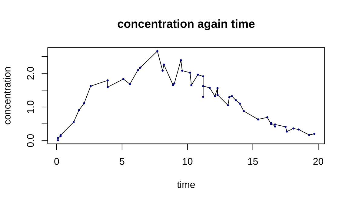
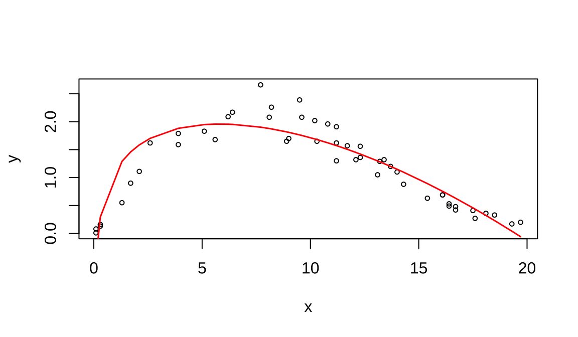
## Note:                    *p<0.1; **p<0.05; ***p<0.01

8.2 药物浓度拟合参数方程

Code

data=read.table('data/nd.txt',header = T)
# 1
plot(data$Time,data$Concentration,type='l',main='concentration again time',
     xlab='time',ylab='concentration')
points(data$Time,data$Concentration,pch=20,cex=0.5,col="blue4")

\[y=log(c)+(b-1)*log(\frac{x}{a})-(x/a)^b\]

Code

# 2
x <- data$Time
y <- data$Concentration
# Fit the model using nls
fit <- nls(y ~ log(c) + (b-1)*log(x/a) - (x/a)^b, 
           start = list(c = 10, a = 2, b = 2))
# Print the estimated parameters
summary(fit)

## 
## Formula: y ~ log(c) + (b - 1) * log(x/a) - (x/a)^b
## 
## Parameters:
##   Estimate Std. Error t value Pr(>|t|)    
## c  15.4162     1.0988    14.0   <2e-16 ***
## a   9.7896     0.2607    37.6   <2e-16 ***
## b   1.7001     0.0397    42.8   <2e-16 ***
## ---
## Signif. codes:  
## 0 '***' 0.001 '**' 0.01 '*' 0.05 '.' 0.1 ' ' 1
## 
## Residual standard error: 0.297 on 47 degrees of freedom
## 
## Number of iterations to convergence: 9 
## Achieved convergence tolerance: 1.19e-06

Code

# predict
ynew=log(15.41621) + (1.70005-1)*log(x/9.78956) - (x/9.78956)^1.70005
# plot fit 
plot(x,y,cex=0.6)
lines(x,ynew,col='red',lwd=1.5)

8.3 多余变量

Code

library(haven)
library(foreign)
library(tidyverse)
library(reshape2)
library(boot)
library(glmnet)
FF_wave6_2020v2 <- read_dta("data/FF_wave6_2020v2.dta")

Code

ind=c('p6b5','p6b10', 'p6b35', 'p6b55', 'p6b60', 'p6c21', 'p6f32', 'p6f35', 'p6h74', 'p6h102', 'p6i7', 'p6i8', 'p6i11', 'p6j37', 'k6b21a', 'k6b22a', 'k6c1', 'k6c4e', 'k6c28', 'k6d37', 'k6f63', 'ck6cbmi', 'k6d10')
mydata=FF_wave6_2020v2[,ind]
# mydata=lapply(mydata,as.numeric)
# mydata=as.data.frame(mydata)
mydata[mydata<0]=NA
new=na.omit(mydata)
dim(new)

## [1] 488  23

Code

names(new)[1]='Depression'
new=new %>% mutate(Depression=ifelse(Depression==2,0,1))

8.3.1 后退法

Code

mod_glm1=glm(Depression ~ 1,new,family='binomial')
model_selected=step(mod_glm1,scope =list(upper=paste0('~',paste0(ind[-1],collapse ="+")),lower=~1) ,trace = F,direction ="forward")
model_selected$coefficients

## (Intercept)       p6b55       p6b10      k6b21a 
##    -4.04029     1.49803    -1.78293     0.74077 
##       p6f32       p6c21       p6j37       k6c4e 
##    -0.59864     0.86352    -0.76027     0.53427 
##     ck6cbmi 
##     0.04254

Code

summary(model_selected)

## 
## Call:
## glm(formula = Depression ~ p6b55 + p6b10 + k6b21a + p6f32 + p6c21 + 
##     p6j37 + k6c4e + ck6cbmi, family = "binomial", data = new)
## 
## Deviance Residuals: 
##    Min      1Q  Median      3Q     Max  
## -2.120  -0.408  -0.290  -0.207   3.008  
## 
## Coefficients:
##             Estimate Std. Error z value Pr(>|z|)    
## (Intercept)  -4.0403     1.9312   -2.09   0.0364 *  
## p6b55         1.4980     0.2533    5.91  3.3e-09 ***
## p6b10        -1.7829     0.4517   -3.95  7.9e-05 ***
## k6b21a        0.7408     0.2337    3.17   0.0015 ** 
## p6f32        -0.5986     0.3881   -1.54   0.1229    
## p6c21         0.8635     0.4293    2.01   0.0443 *  
## p6j37        -0.7603     0.4258   -1.79   0.0742 .  
## k6c4e         0.5343     0.3017    1.77   0.0765 .  
## ck6cbmi       0.0425     0.0245    1.74   0.0819 .  
## ---
## Signif. codes:  
## 0 '***' 0.001 '**' 0.01 '*' 0.05 '.' 0.1 ' ' 1
## 
## (Dispersion parameter for binomial family taken to be 1)
## 
##     Null deviance: 347.79  on 487  degrees of freedom
## Residual deviance: 253.42  on 479  degrees of freedom
## AIC: 271.4
## 
## Number of Fisher Scoring iterations: 6

Code

CI=confint(model_selected)
d=CI[CI[,1]>0,]
data.frame(name=rownames(d),low=d[,1],upr=d[,2],estimate=rowMeans(d)) %>% 
  group_by(name)%>% 
  ggplot(mapping=aes(y=estimate, x=name)) +
  geom_point() +
  geom_errorbar(aes(ymin = low, ymax = upr), width=.4,col='red')+
  labs(title="A coefficient greater than zero and its confidence interval",
       y="estimate", 
       x="Figure 1: Estimate")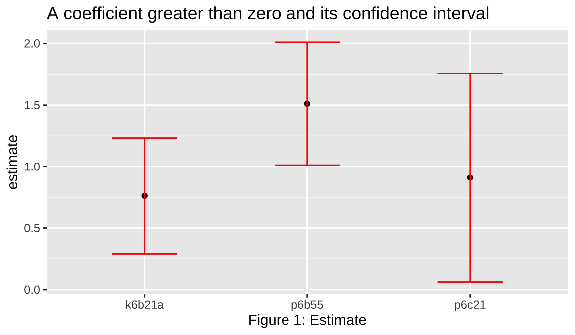

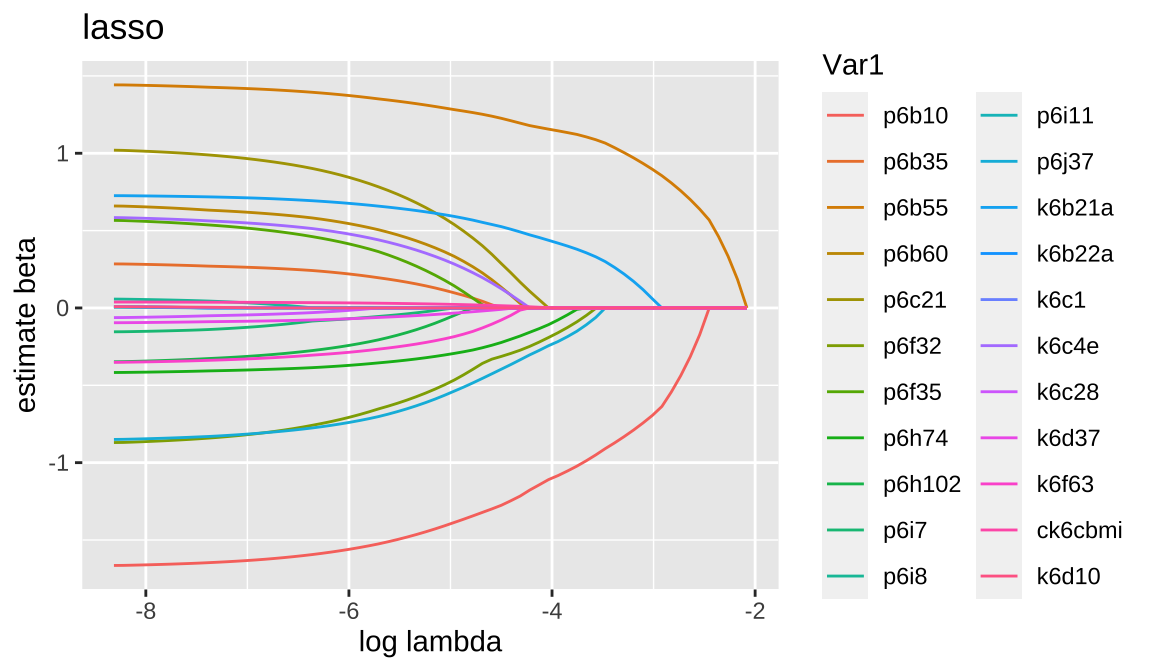
8.3.2 lasso

Code

y=as.integer(new[,1]$Depression)
x=as.matrix(new[,-1])
f1=glmnet(x,y,family = 'binomial',nlambda = 100,alpha = 1)
la=f1$lambda
co=f1$beta
ll1=as.matrix(co)
dim(ll1)

## [1] 22 68

Code

colnames(ll1)=log(la)
ladat=melt(ll1)
ggplot(ladat,aes(x=Var2,y=value,col=Var1))+geom_line()+
    labs(title="lasso",
       y="estimate beta", 
       x="log lambda")

Code

cvfit=cv.glmnet(x,y)
lasso_coef = predict(f1, type = "coefficients", s = cvfit$lambda.min)
lasso_coef

## 23 x 1 sparse Matrix of class "dgCMatrix"
##                   s1
## (Intercept) -1.94241
## p6b10       -1.05411
## p6b35        .      
## p6b55        1.13370
## p6b60        .      
## p6c21        .      
## p6f32       -0.12648
## p6f35        .      
## p6h74       -0.04463
## p6h102       .      
## p6i7         .      
## p6i8         .      
## p6i11        .      
## p6j37       -0.18554
## k6b21a       0.40028
## k6b22a       .      
## k6c1         .      
## k6c4e        .      
## k6c28        .      
## k6d37        .      
## k6f63        .      
## ck6cbmi      .      
## k6d10        .

The coefficients obtained with the Lasso procedure are similar to the coefficients obtained with the forward procedure, but there are some differences. The Lasso tends to shrink coefficients towards zero, which can result in some coefficients being set to zero even if they were significant in the forward procedure.

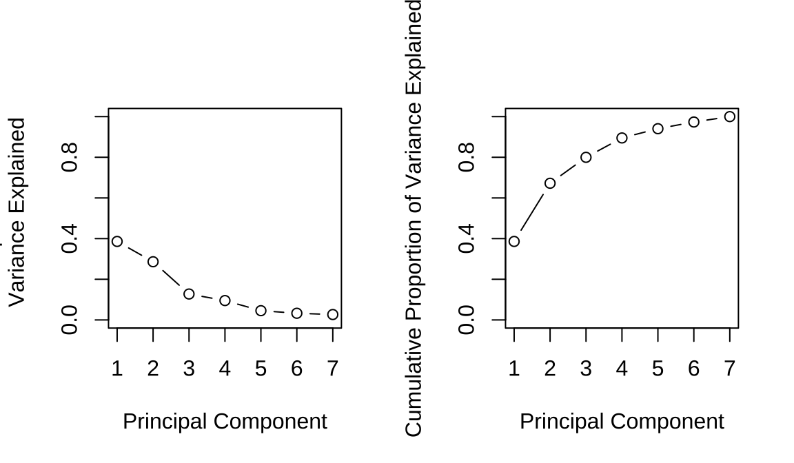
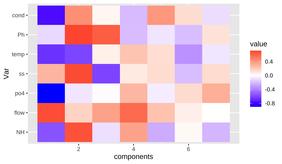
8.3.3 偏最小二乘

Code

library(tidyverse)
library(reshape2)
datn=readxl::read_xlsx('data/pzx.xlsx')
datn$NH=gsub(",",".",datn$NH)
datn$NH=as.numeric(datn$NH)
dat=scale(datn)
X <- dat[,-1] #对原始数据进行标准化处理
pr.out <- prcomp(X)
summary(pr.out)

## Importance of components:
##                          PC1   PC2   PC3    PC4    PC5
## Standard deviation     1.644 1.415 0.945 0.8167 0.5646
## Proportion of Variance 0.386 0.286 0.128 0.0953 0.0455
## Cumulative Proportion  0.386 0.672 0.800 0.8950 0.9406
##                           PC6    PC7
## Standard deviation     0.4796 0.4314
## Proportion of Variance 0.0328 0.0266
## Cumulative Proportion  0.9734 1.0000

Code

pr.var <- pr.out$sdev^2 
pve <- pr.var/sum(pr.var) 
cumsum(pve)

## [1] 0.3861 0.6722 0.7998 0.8950 0.9406 0.9734 1.0000

Code

par(mfrow = c(1, 2))
plot(pve, xlab = "Principal Component", ylab = "Proportion of
  Variance Explained", ylim = c(0, 1), type = "b")
plot(cumsum(pve), xlab = "Principal Component", ylab = "Cumulative Proportion of Variance Explained", ylim = c(0, 1), type = "b")

Code

pca=pr.out$rotation %*% diag(pr.out$sdev)#factor loadings
Score=pr.out$x

Code

##载荷可视化
melt(pca)%>% 
  ggplot(mapping = aes(x =Var2 , y = Var1, fill = value)) + 
  geom_tile() + scale_fill_gradient2(mid="white",low = 'blue', high = 'red') + 
  xlab('components')+ylab('Var')

Code

pcd_dat=cbind(y=dat[,1],Score[,1:3])
pcd_dat=as.data.frame(pcd_dat)
set.seed(123)
ind=sample(1:nrow(dat),0.7*nrow(dat))
train=pcd_dat[ind,]
test=pcd_dat[-ind,]
modpca=lm(y~.,train)
## 对训练数据的拟合程度R2
summary(modpca)

## 
## Call:
## lm(formula = y ~ ., data = train)
## 
## Residuals:
##     Min      1Q  Median      3Q     Max 
## -2.4387 -0.3243  0.0846  0.3825  1.5888 
## 
## Coefficients:
##             Estimate Std. Error t value Pr(>|t|)    
## (Intercept)  -0.0015     0.0594   -0.03    0.980    
## PC1          -0.3388     0.0364   -9.31  1.2e-15 ***
## PC2           0.4209     0.0445    9.46  5.4e-16 ***
## PC3          -0.1892     0.0623   -3.04    0.003 ** 
## ---
## Signif. codes:  
## 0 '***' 0.001 '**' 0.01 '*' 0.05 '.' 0.1 ' ' 1
## 
## Residual standard error: 0.64 on 113 degrees of freedom
## Multiple R-squared:  0.604,  Adjusted R-squared:  0.594 
## F-statistic: 57.5 on 3 and 113 DF,  p-value: <2e-16

Code

#用于还原数据
sdd=as.vector(sapply(datn,sd))
mean=as.vector(sapply(datn,mean))
coef(modpca)

## (Intercept)         PC1         PC2         PC3 
##   -0.001503   -0.338799    0.420850   -0.189184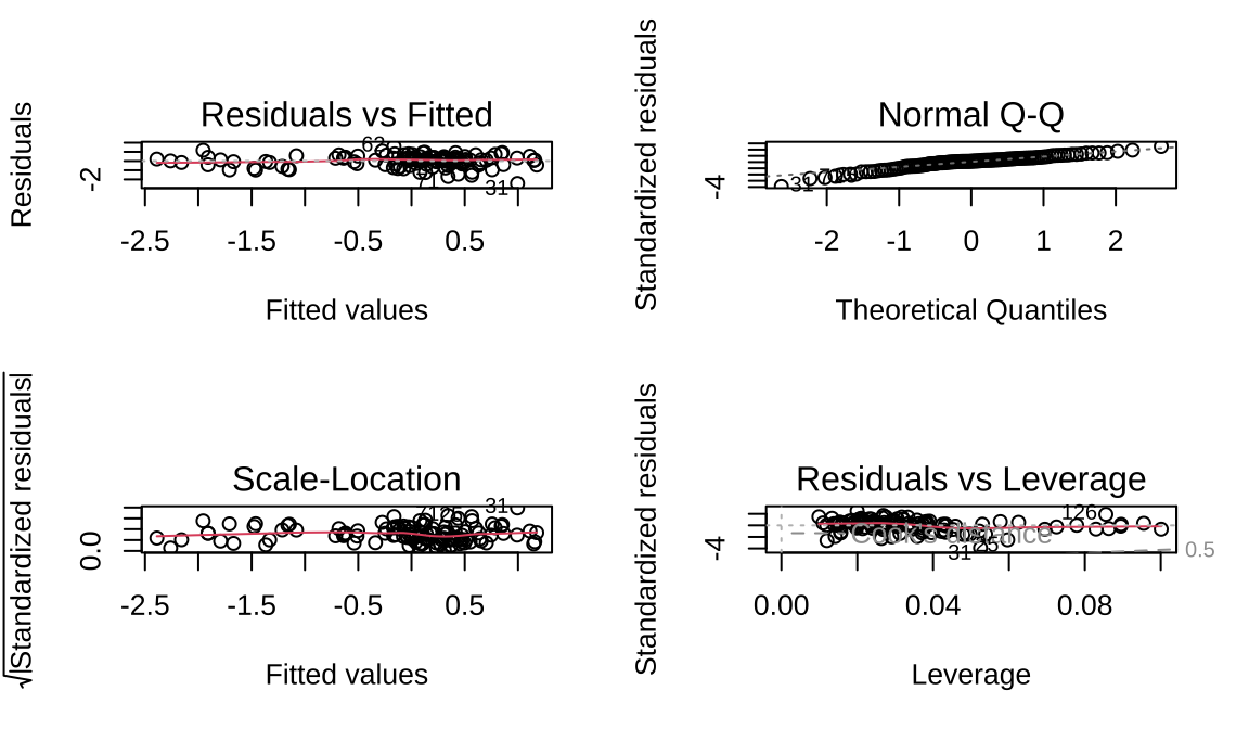

Code

par(mfrow=c(2,2))
plot(modpca)

Code

par(mfrow=c(1,1))
#预测
par(mfrow=c(1,2))
pre1=predict(modpca,test)
plot(1:nrow(test),pre1,type='l')
points(1:nrow(test),pre1)
lines(1:nrow(test),test$y,col=2)
points(1:nrow(test),test$y,pch=3,col=2)

plot(test$y,pre1)
abline(0,1,col=2)

Code

par(mfrow=c(1,1))
#预测残差平方和
sum((pre1-test$y)^2)

## [1] 30.27

Code

# RMSE
sqrt(sum((pre1-test$y)^2)/nrow(test))

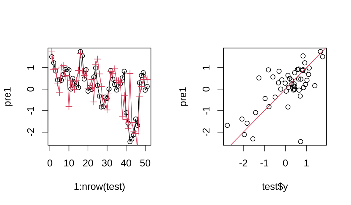
## [1] 0.7703

Code

coe1=pca[,1:3]%*%coef(modpca)[-1]#主成分还原

#标准化还原
pcab=sdd[1]*as.vector(coe1)/sdd[-1]
pacb0<-sum(-sdd[1]*coe1*mean[-1]/sdd[-1])+mean[1]+coef(modpca)[1]*sdd[1]
c(pacb0,pcab)

## (Intercept)                                     
##  -324.45790     1.59843    -0.01102     7.75341 
##                                                 
##     0.05608    -1.46149    41.60263     0.05822

Code

sum(datn[1,-1]*c(pcab))+pacb0

## (Intercept) 
##       221.6

Code

# install.packages("pls")
library(pls)
dat=as.data.frame(dat)
train2=dat[ind,]
test2=dat[-ind,]
pls1 <- plsr(scod~.,data=train2,validation='LOO',jackknife=TRUE,
             method='widekernelpls')
summary(pls1,what='all')

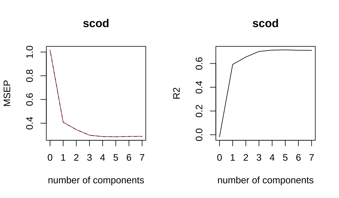
## Data:    X dimension: 117 7 
##  Y dimension: 117 1
## Fit method: widekernelpls
## Number of components considered: 7
## 
## VALIDATION: RMSEP
## Cross-validated using 117 leave-one-out segments.
##        (Intercept)  1 comps  2 comps  3 comps  4 comps
## CV           1.009   0.6392   0.5881   0.5468   0.5361
## adjCV        1.009   0.6391   0.5880   0.5467   0.5360
##        5 comps  6 comps  7 comps
## CV      0.5343   0.5373   0.5378
## adjCV   0.5341   0.5372   0.5376
## 
## TRAINING: % variance explained
##       1 comps  2 comps  3 comps  4 comps  5 comps
## X       34.20    65.64    76.99    86.97    94.35
## scod    61.72    68.49    73.72    74.91    75.22
##       6 comps  7 comps
## X       98.05   100.00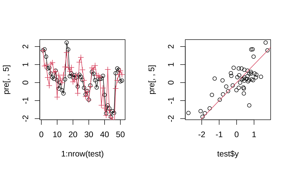
## scod    75.22    75.22

Code

pls3 <- plsr(scod~.,data=dat,ncomp=5,validation='LOO',jackknife=TRUE)
coef(pls3)

## , , 5 comps
## 
##          scod
## NH    0.42900
## flow  0.10748
## po4   0.46516
## ss    0.06142
## temp -0.41347
## Ph   -0.20848
## cond  0.28241

Code

par(mfrow = c(1, 2))
validationplot(pls1, val.type = 'MSEP')
validationplot(pls1, val.type = 'R2')

Code

pre=predict(pls3,test2)
summary(pls3)

## Data:    X dimension: 168 7 
##  Y dimension: 168 1
## Fit method: kernelpls
## Number of components considered: 5
## 
## VALIDATION: RMSEP
## Cross-validated using 168 leave-one-out segments.
##        (Intercept)  1 comps  2 comps  3 comps  4 comps
## CV           1.003    0.672   0.6310   0.6027   0.5918
## adjCV        1.003    0.672   0.6309   0.6027   0.5917
##        5 comps
## CV      0.5900
## adjCV   0.5899
## 
## TRAINING: % variance explained
##       1 comps  2 comps  3 comps  4 comps  5 comps
## X       34.14    60.21    76.09    82.90    92.77
## scod    56.95    63.08    66.90    68.76    68.92

Code

pre[,,5]

##         1         2         3         9        10 
##  1.789077  1.847178  1.439600  0.783259  0.822152 
##        15        18        19        20        28 
##  0.504052  0.287674  0.208961  0.661821  0.120597 
##        29        33        45        48        49 
## -0.330300 -0.003067 -0.420008 -0.604028  0.178544 
##        56        57        58        59        61 
##  2.221033  1.837313  0.356347  0.503241  0.297697 
##        66        70        73        77        80 
##  0.405937  0.286347 -0.220258  0.438075  0.323224 
##        82        85        88        93        96 
##  0.140048 -0.287251 -0.652196 -0.473903 -0.951519 
##        98       100       104       105       110 
## -0.158494  0.592749  0.499284  0.131835 -0.271080 
##       112       113       119       120       122 
##  0.216270  0.189855  0.223635  0.373624 -0.682756 
##       125       127       128       130       136 
## -1.701492 -1.265795 -1.431167 -1.898188 -1.584910 
##       142       147       148       150       155 
## -1.685985  0.520509  0.784047  0.710252  0.069777 
##       162 
##  0.109711

Code

par(mfrow=c(1,2))
plot(1:nrow(test),pre[,,5],type='l')
points(1:nrow(test),pre[,,5])
lines(1:nrow(test),test$y,col=2)
points(1:nrow(test),test$y,pch=3,col=2)
plot(test$y,pre[,,5])
abline(0,1,col=2)

Code

par(mfrow=c(1,1))
## 对预测数据的预测能力
# 残差平方和
sum((pre[,,5]-test2$scod)^2)

## [1] 21.97

Code

# RMSE
sqrt(sum((pre[,,5]-test2$scod)^2)/nrow(test2))

## [1] 0.6563

Code

# 系数还原
coe=coef(pls3)
coe=as.vector(coe)
b=sdd[1]*as.vector(coe)/sdd[-1]
b0<-sum(-sdd[1]*coe*mean[-1]/sdd[-1])+mean[1]
c(b0,b)

## [1] 508.325179   1.409096   0.005195  13.170441
## [5]   0.011127 -15.633216 -39.297392   0.038004

Code

#验证
sum(datn[1,-1]*c(b))+b0

## [1] 212.7

Code

datn[1,1]

## # A tibble: 1 × 1
##    scod
##   <dbl>
## 1   212

Code

## 对训练数据的拟合程度
SST=sum((train2$scod-mean(train2$scod))^2)
SSE=sum((pls3$residuals[,,5])^2)
(SST-SSE)/SST

## [1] 0.5569

第 8 章 回归

8.1 有序glm

8.2 药物浓度拟合参数方程

8.3 多余变量

8.3.1 后退法

8.3.2 lasso

8.3.3 偏最小二乘

第 8 章回归