第 7 章 聚类
## [1] 88 108 55 77 56 62 1 79 64 14Code
##
## Call:
## hclust(d = dist(irisdata[, -5]), method = "single")
##
## Cluster method   : single
## Distance         : euclidean
## Number of objects: 140##
## Call:
## hclust(d = dist(irisdata[, -5]), method = "complete")
##
## Cluster method : complete
## Distance : euclidean
## Number of objects: 140##
## Call:
## hclust(d = dist(irisdata[, -5]), method = "average")
##
## Cluster method : average
## Distance : euclidean
## Number of objects: 140##
## setosa versicolor virginica
## 1 0 37 3
## 2 48 0 0
## 3 0 6 467.1 1 Data Importing
Code
##   age anaemia creatinine_phosphokinase diabetes
## 1  75       0                      582        0
## 2  55       0                     7861        0
## 3  65       0                      146        0
## 4  50       1                      111        0
## 5  65       1                      160        1
## 6  90       1                       47        0
##   ejection_fraction high_blood_pressure platelets
## 1                20                   1    265000
## 2                38                   0    263358
## 3                20                   0    162000
## 4                20                   0    210000
## 5                20                   0    327000
## 6                40                   1    204000
##   serum_creatinine serum_sodium sex smoking time
## 1              1.9          130   1       0    4
## 2              1.1          136   1       0    6
## 3              1.3          129   1       1    7
## 4              1.9          137   1       0    7
## 5              2.7          116   0       0    8
## 6              2.1          132   1       1    8
##   DEATH_EVENT
## 1           1
## 2           1
## 3           1
## 4           1
## 5           1
## 6 1## [1] 299 13##
## 0 1
## 203 967.2 2 Clustering
7.2.1 2.0 pre-processing
Code
##  [1] "age"
##  [2] "anaemia"
##  [3] "creatinine_phosphokinase"
##  [4] "diabetes"
##  [5] "ejection_fraction"
##  [6] "high_blood_pressure"
##  [7] "platelets"
##  [8] "serum_creatinine"
##  [9] "serum_sodium"
## [10] "sex"
## [11] "smoking"
## [12] "time"
## [13] "DEATH_EVENT"7.2.2 2.1 K-means
Find groups of similar cases in your data set using k-means clustering. We analyzed the case k equal to 2 − 15 directly on the original data.
Code
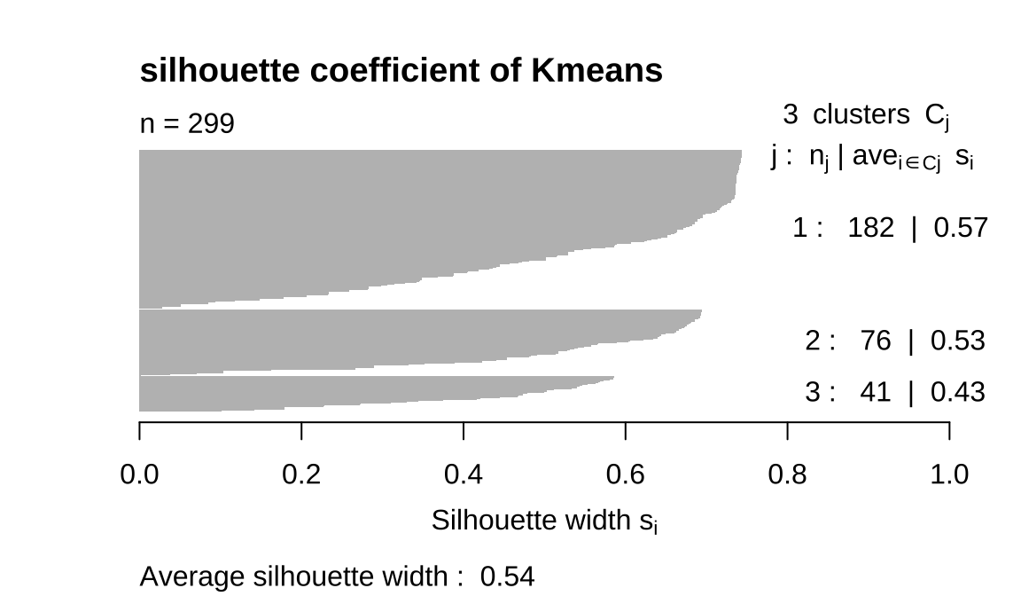
1.Using the Silhouette coefficient,We want to find the point with the largest silhouette coefficient, which shows the relationship between the within-group distance and the between-group distance.
Code
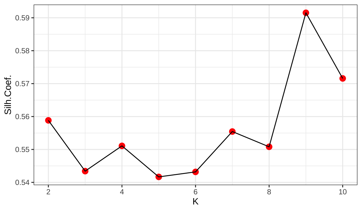 Select K=4 which is the highest average silhouette coefficient.
2.Using the Elbow method,We need to find the obvious turning point.
Code
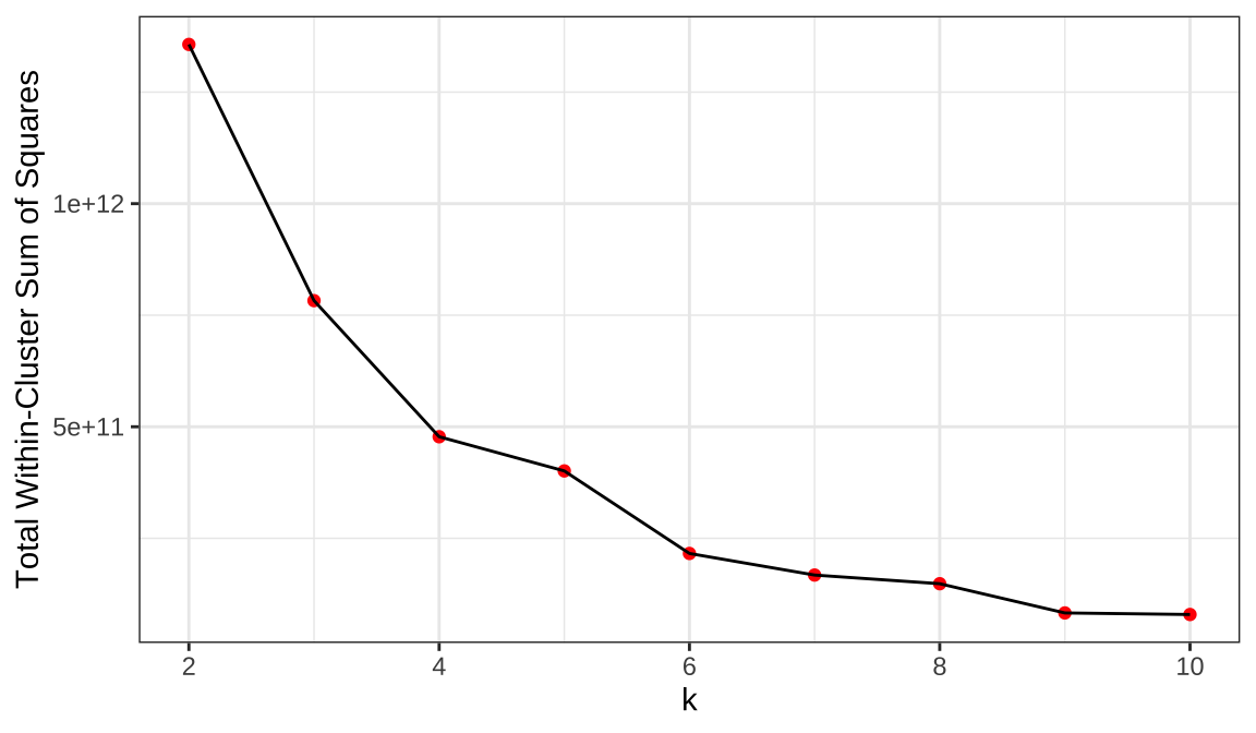 Select K at the inflection point (K=4).
The most appropriate number of clusters is four in 2-6.It is the category with the largest silhouette coefficient and is clearly turning Using the Elbow method
7.2.4 2.3 PAM (Gower)
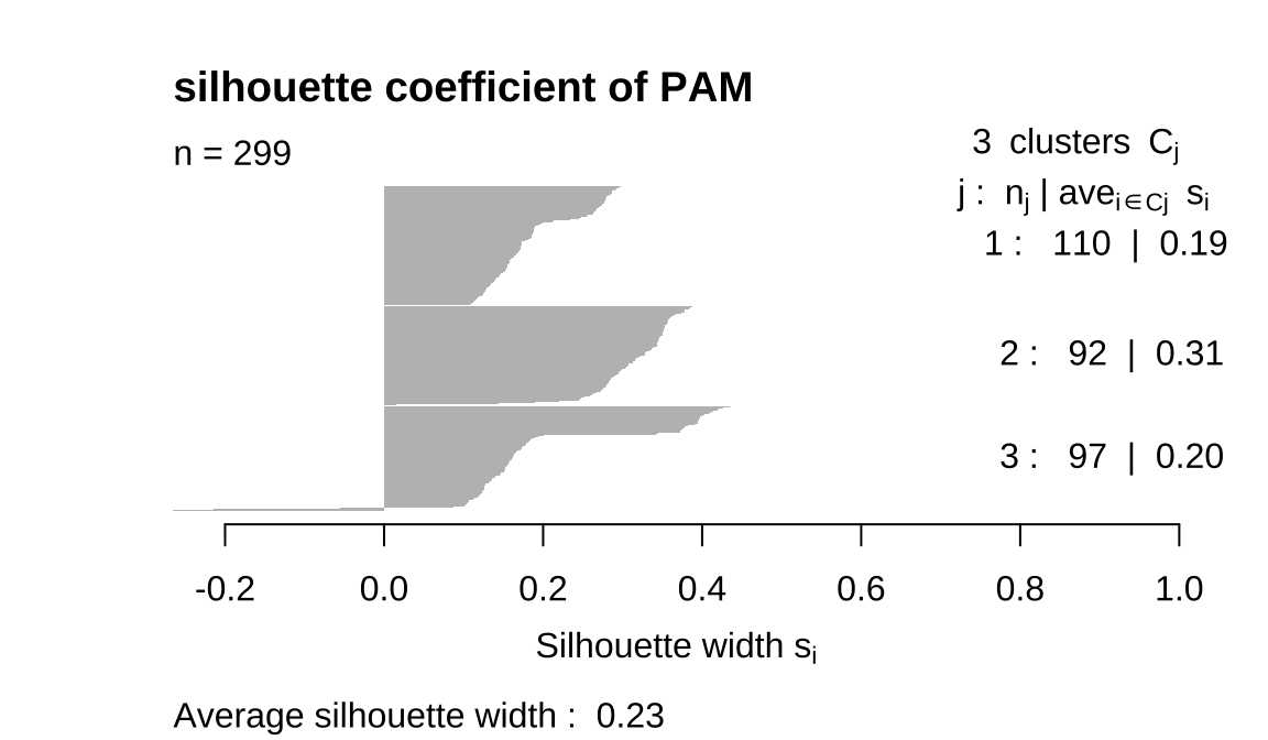
PAM is a medoid-based clustering algorithm that attempts to partition a dataset into a predetermined number of clusters, where the center of each cluster is the actual observation (medoid) in the dataset. Unlike k-means clustering, PAM uses medoids instead of means as cluster center points, which makes PAM more robust to handling outliers. The PAM function is used to perform PAM clustering in a given R code. The daisy() function is used to compute the Gower similarity matrix of the dataset, which contains a measure of similarity between samples. The Gower similarity measure is suitable for mixed data types (a combination of numeric and categorical variables) because it takes into account distance measures for different types of variables.
Code
##
##   1   2   3
## 110  92  97
7.3 3 Describe the clusters you found with PAM
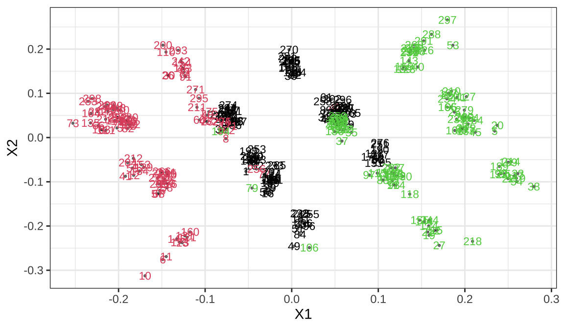
The clusplot function is often used for visualizing clusters, There is an intersection of the three categories
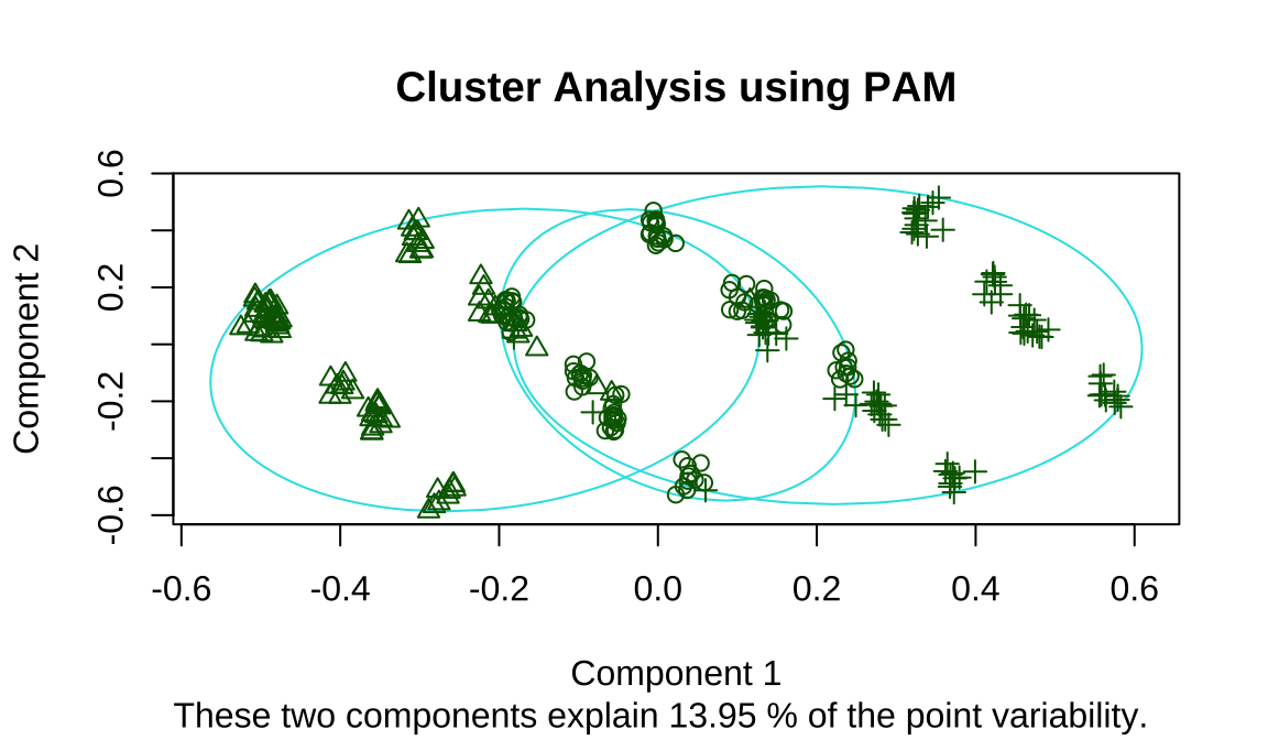
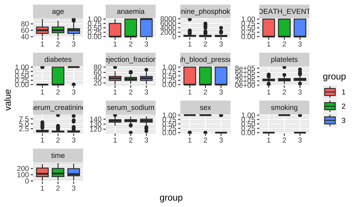
- the 3 cluster means (center). We can focus on variables that are significantly different.like 3 is high anaemia.
##   Group.1   age anaemia creatinine_phosphokinase
## 1       1 61.63  0.2545                    681.2
## 2       2 60.77  0.3261                    599.6
## 3       3 59.99  0.7320                    452.3
##   diabetes ejection_fraction high_blood_pressure
## 1   0.2273             37.64              0.3727
## 2   0.2935             37.05              0.3043
## 3   0.7526             39.57              0.3711
##   platelets serum_creatinine serum_sodium    sex
## 1    249258            1.420        136.6 0.7727
## 2    264655            1.350        136.7 0.9783
## 3    278118            1.406        136.6 0.1959
##   smoking  time DEATH_EVENT
## 1 0.00000 129.8      0.3545
## 2 1.00000 129.0      0.3043
## 3 0.04124 131.9      0.2990
Further analysis of sample distribution for each class using box plots reveals that the age of sample 3 is relatively low. Sample 3 is mostly female, and sample 2 is mostly associated with smoking.
Code
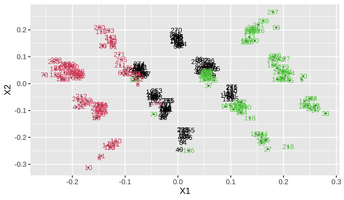
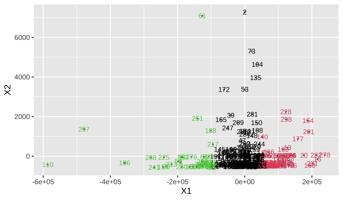
Classical multidimensional scaling (MDS) of a data matrix. Also known as principal coordinates analysis,We’re going to convert this to two dimensional coordinates and look at the distribution
Code
7.4 4 Clustering evaluation and comparison
Code
Code
Code
Code
 - The comparison reveals that 4 K-means has the best silhouette coefficient,
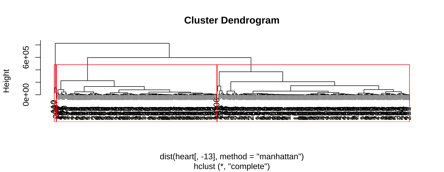
Hierarchical clustering has three classes but the sample size of one class is too small to be considered outlier. PAM three classes are fairly uniform, but we saw earlier that it overlaps.
- The comparison reveals that 4 K-means has the best silhouette coefficient,
Hierarchical clustering has three classes but the sample size of one class is too small to be considered outlier. PAM three classes are fairly uniform, but we saw earlier that it overlaps.
- We convert the distance to coordinates, but since the distance matrix calculation is different, we need to think about which cluster is better
7.5 5 Anomaly detection
Our analysis is based on the simple Euclidean distance, measured on the raw data
7.5.1 LOF
k=3,LOF>4,This method counted 17 samples as abnormal.We show the details of these samples, and the mean comparison of the population can show its characteristics
Code
## [1] 17## [1] 239 254 60 63 97 2 245 107 259 167 203 244
## [13] 17 158 53 169 296## age anaemia creatinine_phosphokinase diabetes
## 239 65 1 720 1
## 254 70 0 88 1
## 60 72 0 364 1
## 63 55 0 109 0
## 97 63 1 514 1
## 2 55 0 7861 0
## 245 54 0 582 1
## 107 55 0 748 0
## 259 45 1 66 1
## 167 53 0 196 0
## 203 70 0 97 0
## 244 73 1 1185 0
## 17 87 1 149 0
## 158 50 0 250 0
## 53 60 0 3964 1
## 169 65 0 582 1
## 296 55 0 1820 0
## ejection_fraction high_blood_pressure platelets
## 239 40 0 257000
## 254 35 1 236000
## 60 20 1 254000
## 63 35 0 254000
## 97 25 1 254000
## 2 38 0 263358
## 245 38 0 264000
## 107 45 0 263000
## 259 25 0 233000
## 167 60 0 220000
## 203 60 1 220000
## 244 40 1 220000
## 17 38 0 262000
## 158 25 0 262000
## 53 62 0 263358
## 169 40 0 270000
## 296 38 0 270000
## serum_creatinine serum_sodium sex smoking time
## 239 1.0 136 0 0 210
## 254 1.2 132 0 0 215
## 60 1.3 136 1 1 59
## 63 1.1 139 1 1 60
## 97 1.3 134 1 0 83
## 2 1.1 136 1 0 6
## 245 1.8 134 1 0 213
## 107 1.3 137 1 0 88
## 259 0.8 135 1 0 230
## 167 0.7 133 1 1 134
## 203 0.9 138 1 0 186
## 244 0.9 141 0 0 213
## 17 0.9 140 1 0 14
## 158 1.0 136 1 1 120
## 53 6.8 146 0 0 43
## 169 1.0 138 0 0 140
## 296 1.2 139 0 0 271
## DEATH_EVENT
## 239 0
## 254 0
## 60 1
## 63 0
## 97 0
## 2 1
## 245 0
## 107 0
## 259 0
## 167 0
## 203 0
## 244 0
## 17 1
## 158 0
## 53 1
## 169 0
## 296 0Code
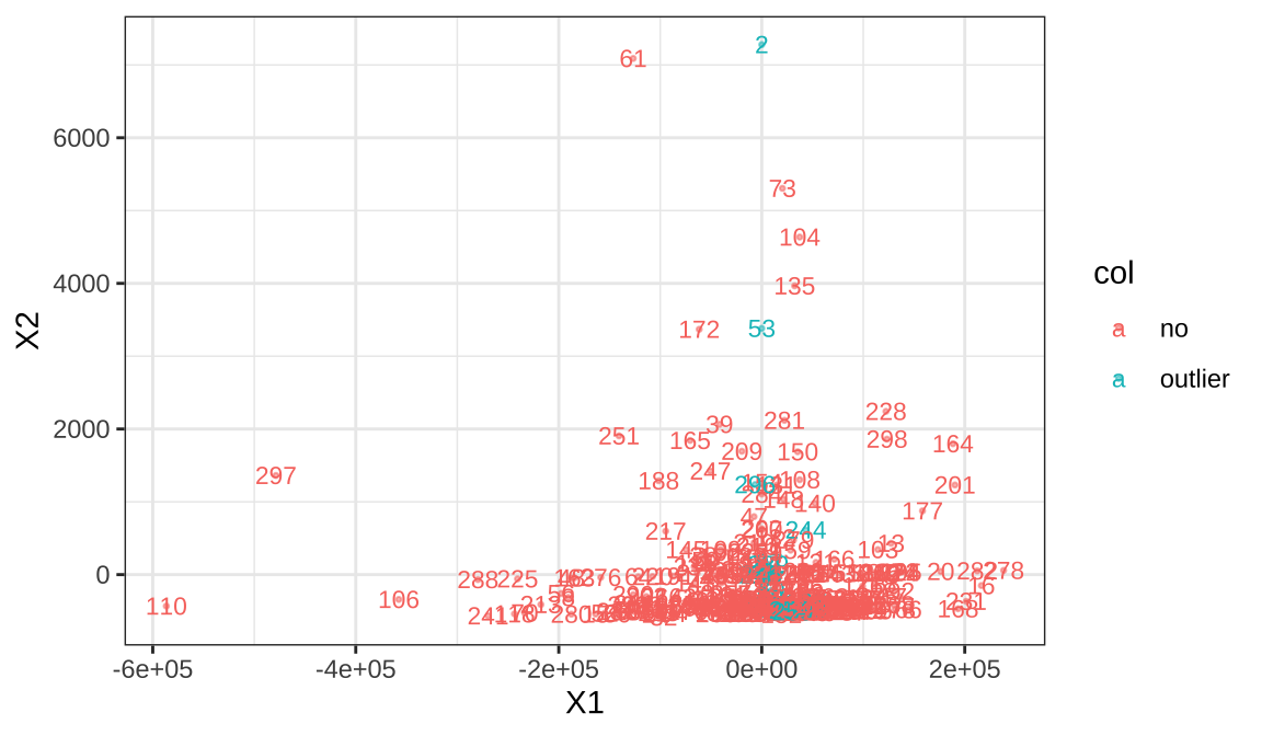
7.5.2 DBSCAN
We measure our detection range as 0.6 times the average distance between point, We counted 19 samples as outliers.
## dbscan Pts=299 MinPts=3 eps=60585
##         0   1 2  3  4  5 6 7 8  9 10 11 12 13 14 15
## border 23   0 0  0  1  0 0 0 1  2  0  0  0  0  0  2
## seed    0 112 6 53 14 30 8 4 6 10 11  3  4  3  5  1
## total 23 112 6 53 15 30 8 4 7 12 11 3 4 3 5 3## [1] 15 16 20 50 52 56 66 70 72 106 110 118
## [13] 177 213 225 231 241 276 278 282 288 297 299## age anaemia creatinine_phosphokinase diabetes
## 15 49 1 80 0
## 16 82 1 379 0
## 20 48 1 582 1
## 50 57 1 129 0
## 52 53 1 91 0
## 56 95 1 371 0
## 66 60 0 68 0
## 70 65 0 113 1
## 72 58 0 582 1
## 106 72 1 328 0
## 110 45 0 292 1
## 118 85 1 102 0
## 177 69 0 1419 0
## 213 78 0 224 0
## 225 58 0 582 1
## 231 60 0 166 0
## 241 70 0 81 1
## 276 45 0 582 0
## 278 70 0 582 1
## 282 70 0 582 0
## 288 45 0 582 1
## 297 45 0 2060 1
## 299 50 0 196 0
## ejection_fraction high_blood_pressure platelets
## 15 30 1 427000
## 16 50 0 47000
## 20 55 0 87000
## 50 30 0 395000
## 52 20 1 418000
## 56 30 0 461000
## 66 20 0 119000
## 70 25 0 497000
## 72 35 0 122000
## 106 30 1 621000
## 110 35 0 850000
## 118 60 0 507000
## 177 40 0 105000
## 213 50 0 481000
## 225 25 0 504000
## 231 30 0 62000
## 241 35 1 533000
## 276 38 1 422000
## 278 38 0 25100
## 282 40 0 51000
## 288 55 0 543000
## 297 60 0 742000
## 299 45 0 395000
## serum_creatinine serum_sodium sex smoking time
## 15 1.00 138 0 0 12
## 16 1.30 136 1 0 13
## 20 1.90 121 0 0 15
## 50 1.00 140 0 0 42
## 52 1.40 139 0 0 43
## 56 2.00 132 1 0 50
## 66 2.90 127 1 1 64
## 70 1.83 135 1 0 67
## 72 0.90 139 1 1 71
## 106 1.70 138 0 1 88
## 110 1.30 142 1 1 88
## 118 3.20 138 0 0 94
## 177 1.00 135 1 1 147
## 213 1.40 138 1 1 192
## 225 1.00 138 1 0 205
## 231 1.70 127 0 0 207
## 241 1.30 139 0 0 212
## 276 0.80 137 0 0 245
## 278 1.10 140 1 0 246
## 282 2.70 136 1 1 250
## 288 1.00 132 0 0 250
## 297 0.80 138 0 0 278
## 299 1.60 136 1 1 285
## DEATH_EVENT
## 15 0
## 16 1
## 20 1
## 50 1
## 52 1
## 56 1
## 66 1
## 70 1
## 72 0
## 106 1
## 110 0
## 118 0
## 177 0
## 213 0
## 225 0
## 231 1
## 241 0
## 276 0
## 278 0
## 282 0
## 288 0
## 297 0
## 299 0Code

no both algorithm Sample 2 appears in both methods
## integer(0)